


 TamoSoft
When planning Wi-Fi for a warehouse or an industrial building, it’s easy to spend a lot of time choosing AP locations and antennas without giving much thought to the height at which the resulting coverage map is calculated. But if the WLAN is supposed to serve both handheld scanners and wireless equipment mounted several meters above the floor, that seemingly minor detail can become pretty important.
A heatmap calculated at 1 m tells you what the model predicts at that height, but it doesn’t tell you if a device mounted at 6 m will see the same signal levels. In TamoGraph 8.5, we added the ability to set the visualization height separately for each map/floor plan, so let’s take a look at when you might want to change it and what you can learn from the result.
Before we begin, let’s clarify something: by “survey height”, I mean the receiver height used for predictive visualization, whereas an actual on-site survey records measurements at the physical location of your Wi-Fi adapter. Changing the prediction height won’t recalculate those measurements as if you had collected them at another elevation.
AP Mounting Height and Visualization Height
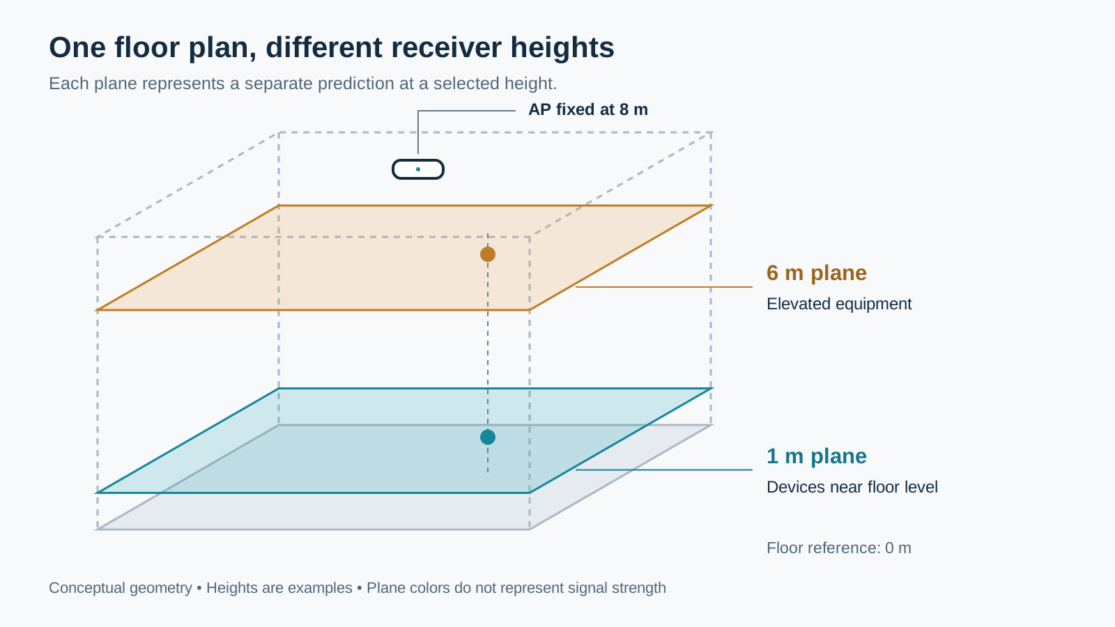
The AP mounting height locates the transmitting antenna in the model, while the visualization height defines the horizontal plane on which TamoGraph calculates the predicted RF conditions. Raising the visualization height from, say, 1 m to 6 m leaves the AP exactly where you put it; you’re simply looking at what the same design predicts at another receiver height. Take a look:
What Happens When the Receiver Moves
Suppose your AP is mounted 8 m above the floor level and the receiver (i.e. the client device) is 5 m away horizontally. At a receiver height of 1 m, the vertical separation is 7 m and the direct path is 8.60 m, whereas raising the receiver to 6 m reduces that path to 5.39 m.
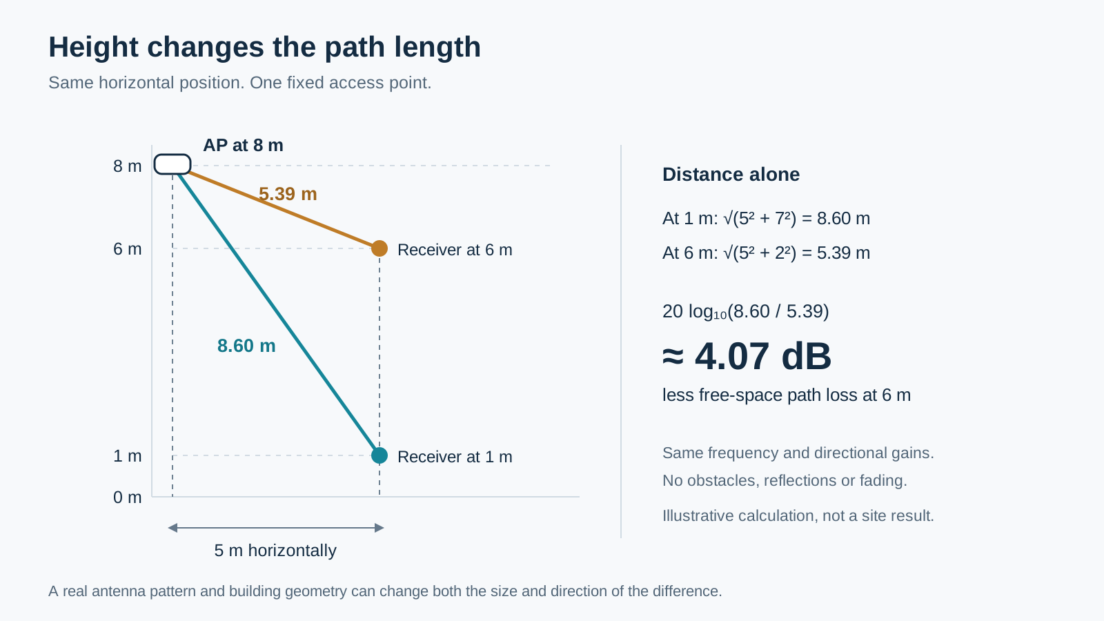
The distance term in the free-space loss equation, 20 log₁₀(d₁ / d₂), gives a difference of about 4 dB, assuming, of course, the same frequency, transmit power, and antenna gains in the relevant directions. No obstacles, reflections, or fading to complicate the picture.
In the real world, warehouses rarely come with a free-space option. When you move the client device, you also change its angle relative to the antenna pattern of the AP in question. Besides, the propagation path may cross shelving, machinery, etc. Reflections and multipath then add further variation, so the distance between the AP and the receiver is just one of the factors that determine RSSI.
Now, let’s add more drama: A device higher up may have a clearer path to one AP while losing a useful path to another, so there is no general rule that higher receiver positions produce better coverage. The calculation explains one reason for a difference, while the antennas and the environment determine what that difference will actually be.
Setting the Visualization Height in TamoGraph
Before version 8.5, TamoGraph displayed predicted coverage on a plane fixed at 1 m above the floor; in the newest version, you can choose the visualization height separately for each map, and the selected height, naturally, is also used when generating reports.
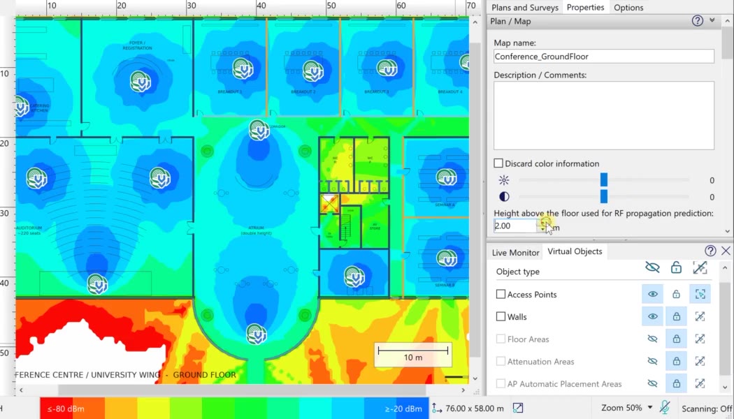
The setting is in the Properties panel, under Plan / Map, where the field labeled “Height above the floor used for RF propagation prediction” applies to the selected map. Enter the receiver height you want to examine and review the updated visualization. The example below shows the setting at 2 m:
If you want to compare two heights, just change the value and the visualization will be recomputed. Alternatively, export the current visualization, change the height on the same map, and export the next result, labeling each image with its height and band so that the comparison is unambiguous. Just keep everything else (AP positions, mounting heights, antenna settings, transmit powers, selected APs, color scale) consistent, because changing several things at once makes it difficult to tell what produced the difference.
Choosing the Heights to Evaluate
I’d start by finding out where the client antennas are during normal operation, whether you’re dealing with desk-based and handheld devices in an office or scanners, vehicle terminals, and fixed equipment in a warehouse. For example, a terminal mounted in a forklift cab will usually remain at cab height when the forks rise, so the height of the load is of little relevance to the antenna’s position.
Equipment that moves vertically calls for several predictions at representative heights across its operating range, while clients working on a mezzanine require you to include that structure in the model and establish the correct floor reference. As for the 1 m and 6 m values in this article, I chose them to illustrate the principle, so they shouldn’t be treated as recommended defaults for your own projects.
You should also consider where each device actually needs service, because a large change in predicted signal level above an unused corner of the building may be far less important than a smaller change along a route that the scanners use throughout the day.
Make the Comparison Useful
When comparing the results, check each height against the project’s requirements, paying attention both to the predicted signal levels and to the availability of alternative APs along important routes. Coverage overlap can help you assess the design, although the heatmap alone won’t tell you how a particular client will roam or how well its application will perform; those questions require testing with the actual devices.
If an important area falls short, try a specific design change, such as moving an AP or adjusting its mounting height or antenna orientation, and then check the predictions at every required client height again. Improving the situation on one plane may change the coverage balance on another, so it’s easy to solve one problem while overlooking a different one.
Keep the height, band, and relevant model assumptions with each exported result. Before generating a report, please don’t forget to check which height is currently selected for every map; otherwise, your report may accidentally use the height you last experimented with, which is not the kind of surprise you want to leave for the guy deploying the network
Checking the Design After Deployment
Even a carefully prepared prediction depends on the quality of its inputs and on the propagation model’s limitations, which is why our RF modeling guide suggests a real survey after deployment. That survey should cover representative client locations and operating conditions, with application performance tested on the intended devices wherever it matters to the job.


